Gappy RegularTimeSeries

Some signals are almost regular: they are sampled at a fixed rate, but have missing samples or chunks of samples. Behavioral streams in neuroscience experiments are a common example: a sensor briefly disconnects or a chunk of data is lost between recording segments.

While such signals can be stored as IrregularTimeSeries, there is a certain benefit to storing signals as RegularTimeSeries: slicing precision. A RegularTimeSeries slice always returns the same number of points for the same window width.

This motivated us to extend the interface of RegularTimeSeries to support gappy regular time series, which keeps that reliable slicing while allowing for missing time points. The main idea, simply, is to represent the missing timestamps with NaNs, while explicitly tracking which samples are real and which are gap-fill.

More on slicing precision

Slicing an IrregularTimeSeries close to real timestamps can return \(N\) or \(N-1\) points depending on floating-point rounding errors. So, in practice, windowed sampling, effectively, behaves non-deterministically. More precisely, this happens because we store timestamps of irregular time series in floating point format (numpy.float64). Slicing involves a search in this floating point space, and comparisons between floating numbers are notoriously unreliable.

A RegularTimeSeries internally represents time as integer indices, where it is easier to control all the messy floating point numerics. As a result, a slice always returns the same number of points for the same window width.

Creating a gappy series

Use RegularTimeSeries.from_gappy_timeseries() when you have regularly-sampled but gappy timestamps and value arrays. Each sample is snapped to a regular grid at sampling_rate, and missing samples are filled with a configurable gap value.

>>> from temporaldata import RegularTimeSeries

>>> # Signal sampled at 1 Hz but a few samples dropped: t = 3, 6, 7
>>> ts = [0., 1., 2., 4., 5., 8., 9.,]
>>> values = [0.1, 0.4, 0.2, 0.1, 0.0, 0.3, 0.5,]

>>> signal = RegularTimeSeries.from_gappy_timeseries(
...     timestamps=ts,
...     values=values,
...     sampling_rate=1.0,
... )

>>> len(signal)
10

>>> signal.timestamps
array([ 0.,  1.,  2.,  3.,  4.,  5.,  6.,  7.,  8.,  9.])

>>> signal.values
array([0.1, 0.4, 0.2, nan, 0.1, 0.0, nan, nan, 0.3, 0.5])

The resulting object behaves like any other RegularTimeSeries, just with some gap-fill values.

Tip

You can customize which gap-fill values are used for different data types. To do this, see the gap_value parameter of from_gappy_timeseries().

Domain

While a contiguous RegularTimeSeries has a contiguous domain, a gappy series carries a non-contiguous domain that excludes the gap regions. For the example above:

>>> signal.domain.start, signal.domain.end
array([0., 4., 8.]), array([3., 6., 10.])

This is \([0, 3) \cup [4, 6) \cup [8, 10)\).

Identifying real vs. gap-fill samples

To help you decipher which samples are real and which are gap-fills, we provide the index_mask() method. It returns a boolean mask marking which positions hold real observations:

>>> signal.index_mask()
array([ True,  True,  True, False,  True,  True, False, False,  True,  True])

>>> # to get back "real" signal values:
>>> signal.values[signal.index_mask()]
array([0.1, 0.4, 0.2, 0.1, 0.0, 0.3, 0.5])

For a contiguous series, index_mask() returns an all-True array.

is_gappy() is another convenient introspection method:

>>> signal.is_gappy()
True

>>> contiguous = RegularTimeSeries(values=[0.1, 0.4, 0.2], sampling_rate=1.0)
>>> contiguous.is_gappy()
False

Slicing

Slicing mostly follows the normal RegularTimeSeries semantics, with two additions specific to gappy series:

• Edge gaps are trimmed. If a slice boundary falls inside a gap, the returned arrays will not begin or end with gap-fill samples. That is, slicing always returns data bracketed by real samples.

• Internal gaps are preserved if needed. Gap-fill samples in the middle of the requested window remain in place; the returned object is itself gappy.

>>> sliced = signal.slice(3.0, 9.0, reset_origin=False)
>>> sliced.timestamps
array([ 4.,  5.,  6.,  7.,  8.])
>>> sliced.values
array([0.1, 0. , nan, nan, 0.3])
>>> sliced.domain.start, sliced.domain.end
array([4., 8.]), array([6., 9.])

Notice that the domain does not start at \(t = 3\), and the gap between \(t = 6\) and \(t = 8\) is preserved.

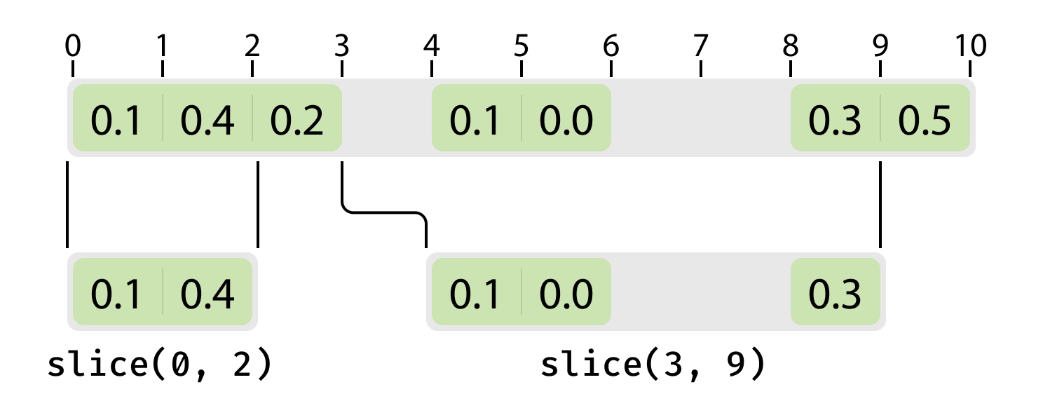
Slicing gappy RegularTimeSeries

A slice that is entirely within a contiguous section is no longer gappy:

>>> sliced = signal.slice(0.0, 2.0, reset_origin=False)
>>> sliced.timestamps
array([ 0.,  1.])
>>> sliced.is_gappy()
False

A slice that falls entirely within a gap returns an empty series:

>>> empty = signal.slice(6.0, 8.0, reset_origin=False)
>>> empty.timestamps
array([])
>>> empty.values
array([])

Conversion to IrregularTimeSeries

to_irregular() drops gap-fill samples and returns an IrregularTimeSeries containing only real observations:

>>> irts = signal.to_irregular()
>>> irts.timestamps
array([0., 1., 2., 4., 5., 8., 9.])
>>> irts.values
array([0.1, 0.4, 0.2, 0.1, 0. , 0.3, 0.5])
>>> irts.domain.start, irts.domain.end
array([0., 4., 8.]), array([3., 6., 10.])

The resulting object’s domain matches the original gappy series’ multi-interval domain, so the gaps remain explicit even after conversion.